Motivation
For the last 5 years, I have been advocating the analysis of k-mer spectra (in short, the frequencies at which different k-mers appear on different datasets) to evaluate genome assemblies. I have been using k-mers for many other analyses too, as do most people doing Bioinformatics. I also train others to perform k-mer analyses and have a long overdue debt to them to write down a more coherent version of the training. So here it goes, with the hope that it gets more people introduced to this simple and straightforward way to analyse sequence data. It is just counting, and everyone can count.

k-mers from a sequence
What is a k-mer anyway? A k-mer is just a sequence of k characters in a string (or nucleotides in a DNA sequence). Now, it is important to remember that to get all k-mers from a sequence you need to get the first k characters, then move just a single character for the start of the next k-mer and so on. Effectively, this will create sequences that overlap in k-1 positions.
So, by way of example, the sequence ATCGATCAC contains the following 3-mers (k-mer of size 3):
Sequence: ATCGATCAC
3-mer #0: ATC
3-mer #1:  TCG
3-mer #2:   CGA
3-mer #3:    GAT
3-mer #4:     ATC
3-mer #5:      TCA
3-mer #6:       CAC
Or, in a nice looking table which we’ll expand later:
| Offset | 0 | 1 | 2 | 3 | 4 | 5 | 6 |
|---|---|---|---|---|---|---|---|
| 3-mer | ATC | TCG | CGA | GAT | ATC | TCA | CAC |
Obviously, we don’t need to use k=3 every time, so here you have the same example with k=4:
Sequence: ATCGATCAC
4-mer #0: ATCG
4-mer #1:  TCGA
4-mer #2:   CGAT
4-mer #3:    GATC
4-mer #4:     ATCA
4-mer #5:      TCAC
So far, so good, so easy. Notice how there are 1 fewer 4-mer than 3-mers in the same sequence. Any sequence of length L will contain L - k + 1 k-mers, which has implications for k-mer analyses when k is close to the length of the sequence. When k << L, as typically happens when we chop the millions or billions of bp of a genome into k-mers with k in the low hundreds or even tens, you can pretend there’s a k-mer at every position in the genome and forget about it.
I hope you can easily imagine the many analyses that can be performed with k-mers, but if not, don’t worry, I will show some along the way).
 Why are k-mers so popular ?
Decomposing a sequence into its k-mers for analysis allows this set of fixed-size chunks to be analysed rather than the sequence, and this can be more efficient. K-mers are very useful in sequence matching (string matching with n-grams has a rich history), and set operations are faster, easier, and there are a lot of readily-available algorithms and techniques to work with them. A simple example: to check if a sequence S comes from organism A or from organism B, assuming the genomes of A and B are known and sufficiently different, we can check if S contains more k-mers present in A or in B. Yes, there are many tools that do just that.
Basically, using k-mers simplifies bioinformatics to counting and comparing whether things are there or not.
Reverse complement and canonical k-mers
*Note: for this section I assume double-strandness is the typical use case. This is a fair assumption, but there will be exceptions
DNA is normally double stranded, with bases paired on the opposite strands and we normally read (or sequence) on either of the two strands. However, we would like to consider every location of the genome once, no matter on which strand we happened to have landed.
In short: if we read the sequence ATCGAC that is an observation for that sequence and its reverse complement GTCGAT to exist in the genome. One appears when reading the genome in one direction and the other on its opposite, we could have sequenced any of them. So for the sake of completeness we should perform all analyses by considering this sequence ATCGAC/GTCGAT.
Luckily, there is a method in k-mer analysis (or in sequence analysis in general) to be sure we always talk about the same sequence in the same way: we can use only the canonical sequence of a k-mer pair, this is the lexicographically smaller of the two reverse complementary sequences. In other words, the one that comes earliest in alphabetical order.
Most k-mer counting tools will either count in canonical k-mers or have an option to switch between canonical and non-canonical. Most of the time canonical counting will be the default. This means if GTCGAT appears it will be counted as ATCGAC. Most of the time this is exactly what we want.
Here are the 3-mers of ATCGATCAC, this time including the reverse complement and the canonical of each 3-mer too.
| Offset | 0 | 1 | 2 | 3 | 4 | 5 | 6 |
|---|---|---|---|---|---|---|---|
| 3-mer | ATC | TCG | CGA | GAT | ATC | TCA | CAC |
| Reverse Complement | GAT | CGA | TCG | ATC | GAT | TGA | GTG |
| Canonical | ATC | CGA | CGA | ATC | ATC | TCA | CAC |
As you can see, in some cases the canonical k-mer appeared in the original sequence, but in other cases it was the reverse complement.
Why do many tools use odd values for k ?
To write a k-mer based tool, we need to account for the relationship within a k-mer and its reverse complement because we don’t know which direction we are reading from. In many tools this relationship is used to detect sequence orientation: if sequence A has the same k-mers as sequence B, in opposite order and in reverse complement, B is in opposite orientation than A. But when using even values of k, a k-mer can be its own reverse complement, which makes it difficult to handle the reverse complements and orientations. This happens when the first half of the sequence is the reverse complement of the second half, as in TCGCGA. A k-mer of odd k (an odd-mer, if you will) can never be its own reverse complement, because the base in the middle of its sequence should be its own complement. Hence, many tools stick to odd values for k.
Distinct, unique, and total k-mers
People that count k-mers talk about unique k-mers, and there is also the total and the distinct counts to keep in mind. All of these can be also done in canonical or non-canonical ways. Sounds confusing? It’s actually not.
Total k-mers are the simplest of all. As we have shown with the example of ATCGATCAC, the amount of k-mers from a sequence varies with k, and that is basically it. ATCGATCAC has 7 total 3-mers and 6 total 4-mers.
Distinct k-mers are counted only once, even if they appear more times, while Unique k-mers are those that appear only once. These two categories of k-mers are greatly affected by counting canonically or not-canonically, because reverse complements in canonical counting are considered the same k-mer.
This is the 3-mer composition for ATCGATCAC again, in non-canonical form, grouping its k-mer occurrences:
| k-mer | Total count | Distinct count | Unique count |
|---|---|---|---|
| ATC | 2 | 1 | 0 |
| TCG | 1 | 1 | 1 |
| CGA | 1 | 1 | 1 |
| GAT | 1 | 1 | 1 |
| TCA | 1 | 1 | 1 |
| CAC | 1 | 1 | 1 |
| Sum | 7 | 6 | 5 |
And this is the 3-mer composition for ATCGATCAC again, but in canonical form:
| Canonical k-mer | Total count | Distinct count | Unique count |
|---|---|---|---|
| ATC (incl. GAT) | 3 | 1 | 0 |
| CGA (incl. TCG) | 2 | 1 | 0 |
| TCA | 1 | 1 | 1 |
| CAC | 1 | 1 | 1 |
| Sum | 7 | 4 | 2 |
As expected, in this canonical counting version TCG has been grouped into CGA, and GAT has been grouped into ATC. So the count has fewer distinct k-mers, and fewer unique k-mers. Canonical counting will always yield fewer (or at most the same), distinct k-mers and unique k-mers.
What makes unique k-mers so special ?
Unique k-mers make analyses simple. For instance, if a k-mer appears only once in a genome, it can be used to check if a particular region of the genome is present or not in a sample, or to check for variation, or as anchor to align other genome’s content, or reads. Unique content within a genome is a good thing, enabling independent analysis of each part of the genome. Genes being usually made up of quite different content than the “repeats” of a genome is the reason why it is in general easier to assemble the genic part of a genome.
Sadly, repetitive content as a concept is poorly defined between biological and computational terms. While in biological terms a loose definition of repeat could be “the stuff between the genes, which is assumed to be similar and low-complexity”, in computational terms it always means “a portion of sequence that appears exactly the same more than one time”. This is why sometimes gene families (groups of very similar genes) are very hard to analyse as they appear multiple times in the genome. At the same time, this dissonance also gives some light at the end of the tunnel in unexpected scenarios: a biologically important repeat may turn out to have a few unique k-mers every time it appears, which in turn may make it a relatively simple region to analyse with the right choice of sequencing technologies and algorithms.
 Counting k-mers in a (small) genome
We will start with an easy example first: the phi-X174 genome has 5386 bp and is a simple non-repetitive genome.
We can use kat hist to count 27-mers on the genome and check how many times each 27-mer appears (we start with k = 27 because KAT uses that as default):
$ kat hist -o phiX.hist phiX.fasta
Checking the phiX.hist histogram (A.K.A. kmer spectrum) file, every 27-mer in the genome appears only once. After the header lines starting with #, every line has a copy number (A.K.A. frequency) and a number of k-mers.
# Title:27-mer spectra for: phiX.fasta
# XLabel:27-mer frequency
# YLabel:# distinct 27-mers
# Kmer value:27
# Input 1:../genomes/phiX.fasta
###
1 5360
2 0
3 0
4 0
...
It is easy to see all 5360 27-mers appear once. Just to be sure we understand the logic, let’s create a file where all the phi-X genome appears twice, count the 27-mers and check the spectrum file.
$ cat phiX.fasta phiX.fasta > phiX_twice.fasta
$ kat hist -o phiX_twice.hist phiX_twice.fasta
# Title:27-mer spectra for: phiX_twice.fasta
# XLabel:27-mer frequency
# YLabel:# distinct 27-mers
# Kmer value:27
# Input 1:phiX_twice.fasta
###
1 0
2 5360
3 0
4 0
...
Now all 5360 27-mers appear twice. With the basics done, it is time to get into the most popular question on k-mer based analysis.
Choosing k: the size of the universe and specificity vs. sensitivity
Choosing k is not a trivial topic on k-mer analysis. Using a k that is too small will result in many unrelated sequences being composed of the same k-mers, in a textbook case of specificity loss because there being very few possible k-mers of that size. In the extreme of the small k, k=1 only distinguishes two canonical k-mers: A and C. 1-mer analysis is incredibly popular in biology, but it is best known by the name of GC content analysis. On the other hand, using extremely large k values would sacrifice many of the benefits and sensitivity of k-mer analyses in the first place, such as decomposing the larger problem into small easy to solve exact problems that can produce an aggregated solution. This leads to problems in inexact matching which I will describe in future posts.
Knowing how many different k-mers can be constructed at a certain k is a good starting point to make an informed choice of k. We call all possible k-mers the universe, and their count is our size of the universe for k. Since each of the k nucleotides in a k-mer can take any of the A, C, G or T values, the possible combinations of k positions are computed as 4^k. When counting canonical k-mers not every value will be considered, but only those that are canonical. For odd values of k that are half of the k-mers, and the size of the universe becomes (4^k)/2. For even values, due to some k-mers being their own reverse complement, the size is slightly higher at (4^k + 4^(k/2) ) / 2, because these k-mers do not group with others under the same canonical representation. Again, sticking to odd k values makes life simpler, but don’t worry about the formulae too much.
Let’s check now what happens if we change that k value between two carefully chosen values of 9 and 8 in the Phi-X genome (we will discuss how these were chosen soon). For historical reasons (due the to options from Jellyfish, on which KAT is based), KAT uses the -m parameter to set k. If k is small enough, the k-mers will appear more than once in the genome, even for this very simple genome.
So counting with k=9 is done like this:
$ kat hist -o phiX_9mer.hist -m 9 phiX.fasta
Then the phiX_9mer.hist file looks like this:
# Title:9-mer spectra for: phiX.fasta
# XLabel:9-mer frequency
# YLabel:# distinct 9-mers
# Kmer value:9
# Input 1:phiX.fasta
###
1 4972
2 189
3 8
4 1
5 0
6 0
7 0
8 0
9 0
...
Not every 9-mer in the genome appear only once: there are 189 9-mers appearing twice, 8 9-mers appearing trice, and 1 9-mer that appears four times.
So, the number of distinct 9-mers in the phi-X genome is 4972 + 189 + 8 + 1 = 5170, of these only 4972 are unique 9-mers (they only appear once in the genome), and the total number of 9-mers is 4972 * 1 + 189 * 2 + 8 * 3 + 1 * 4 = 5378.
The relationship between total, distinct and unique k-mers in a genome gives insight into its composition and the expected performance of different analyses, and depends on the choice of k , as illustrated by the effect of using 8-mers on phi-X for the same analysis.
$ kat hist -o phiX_8mer.hist -m 8 phiX.fasta
Now the histogram file looks like this:
# Title:8-mer spectra for: phiX.fasta
# XLabel:8-mer frequency
# YLabel:# distinct 8-mers
# Kmer value:8
# Input 1:phiX.fasta
###
1 4159
2 491
3 67
4 8
5 1
6 0
7 0
8 0
9 0
Here, only 4159 8-mers are unique, out of 4726 distinct 8-mers, that are present in the genome’s 5377 total 8-mers.
The full response of the unique, distinct and total k-mer counts for phi-X can be computed by running successive KAT hist analyses, and then a bit of clever awk.
#!/bin/bash
#Counting k-mers for different k on phiX
echo "k,unique,distinct,total"
for k in {1..15}; do
	kat hist -o phiX_$k.hist -m $k phiX.fasta >/dev/null 2>&1
	egrep -v '^#' phiX_$k.hist|awk '{if ($1==1) u=$2; d+=$2; t+=$2*$1;}\
	END{print "'$k',"u","d","t}'
done
Executing this script gives a csv version of the following table:
| k | unique | distinct | total |
|---|---|---|---|
| 1 | 0 | 2 | 5386 |
| 2 | 0 | 10 | 5385 |
| 3 | 0 | 32 | 5384 |
| 4 | 0 | 135 | 5383 |
| 5 | 10 | 506 | 5382 |
| 6 | 434 | 1727 | 5381 |
| 7 | 2295 | 3547 | 5380 |
| 8 | 4159 | 4726 | 5379 |
| 9 | 4972 | 5170 | 5378 |
| 10 | 5254 | 5315 | 5377 |
| 11 | 5346 | 5361 | 5376 |
| 12 | 5369 | 5372 | 5375 |
| 13 | 5374 | 5374 | 5374 |
| 14 | 5373 | 5373 | 5373 |
| 15 | 5372 | 5372 | 5372 |
Which plotted alongside the corresponding sizes of the universe is:
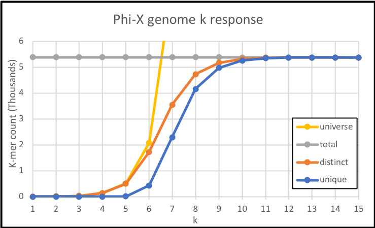
From these results, it is clear there is not a lot to look at for k<5 (see how the unique k-mers are 0), these universes are so small they get completely saturated with the same k-mers over and over again. While frequency analyses like GC content and codon usage can be done there, it is slightly tangential to our topic today.
In the range 5 <= k <= 10, there is a progressive growth on unique and distinct k-mers. Here, the k value makes a difference and will affect the results as the shown in the cherry-picked 9-mer and 8-mer cases earlier.
For k > 10, pretty much every k-mer is unique. As a matter of fact for k >= 13, every k-mer is a unique k-mer.
To make things more interesting, the same analysis can be done for the E. coli genome:
#!/bin/bash
#Counting k-mers for different k on ecoli
echo "k,unique,distinct,total"
for k in {1..31}; do
	kat hist -o ecoli_$k.hist -m $k -h 3000000 ecoli.fasta >/dev/null 2>&1
	egrep -v '^#| 0$' ecoli_$k.hist|awk '{if ($1==1) u=$2; d+=$2; t+=$2*$1;}\
	END{print "'$k',"0+u","d","t}'
done
Note: notice we adjusted the maximum count in the KAT histogram and modified the grep/awk to just skip 0 counts, and there area lot of 0 counts on these files as we are slightly abusing KAT beyond its intended purpose for these examples.
And the corresponding plot looks like this:
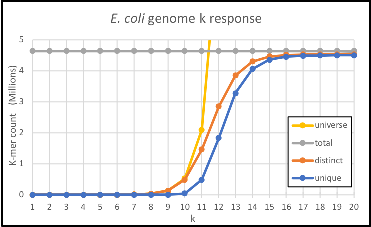
We notice two things straight away: in this larger, relatively more complex genome, there is high saturation of the small universes up to k=10, with all their k-mers fully occupied and no unique k-mers ; and for the higher values of k, the unique and distinct counts do not fully reach the total k-mer number. Even well past desaturation, when the numbers of distinct and unique k-mers separate from the fast-growing size of the universe and become closer to the total k-mers, and up to the last point where k=20, there are still some k-mers that are not unique: these are computational repeats.
Why do many tools use k = 31 ?
31 is the largest odd value of k such that a k-mer can be translated into a 64-bit integer. Most computers nowadays can manipulate 64-bit integers very well and most programming languages will make it easy to work efficiently with 64-bit integers (yes, this has to do with computers using 64-bit architectures). With 31-mers being specific enough that a large number of them are unique both in mammalian-sized genomes (and some more complex genomes too) and in bacterial genome databases, bioinformatics tools just stick to that.
Coming soon…
In future posts we will go over k-mer counting in WGS reads and the read spectrum, onwards to spectra comparisons, and all kinds of k-mer intersection based analyses.
Version History
2018-09-17: initial post.
2018-09-18: corrected small typos and readability.
2018-09-19: more small typos and readability; and clearer explanation of saturation/desaturation on E. Coli genome counting (thanks James Mallet!).
2020-03-04: corrected the number of distinct 8-mers in Phi-X. Thanks @Erdos!!!